External Simulator (Python script)

This example demonstrates the same calibration as Calibration Using LMFIT, but sets up the MATK model as an python script to demonstrate how to use an external simulator. Similar to the External Simulator (FEHM Groundwater Flow Simulator) example, the subprocess call (https://docs.python.org/2/library/subprocess.html) method is used to make system calls to run the model and MATK’s pest_io.tpl_write is used to create model input files with parameters in the correct locations. The pickle package (https://docs.python.org/2/library/pickle.html) is used for I/O of the model results between the external simulator (sine.tpl) and the MATK model.

%matplotlib inline
# Calibration example modified from lmfit webpage
# (http://cars9.uchicago.edu/software/python/lmfit/parameters.html)
# This example demonstrates how to calibrate with an external code
# The idea is to replace `python sine.py` in run_extern with any
# terminal command to run your model.
import sys,os
import numpy as np
from matplotlib import pyplot as plt
from multiprocessing import freeze_support
from subprocess import Popen,PIPE,call
from matk import matk, pest_io
import cPickle as pickle

def run_extern(params):
    # Create model input file
    pest_io.tpl_write(params,'../sine.tpl','sine.py')
    # Run model
    ierr = call('python sine.py', shell=True)
    # Collect model results
    out = pickle.load(open('sine.pkl','rb'))
    return out

# create data to be fitted
x = np.linspace(0, 15, 301)
np.random.seed(1000)
data = (5. * np.sin(2 * x - 0.1) * np.exp(-x*x*0.025) +
        np.random.normal(size=len(x), scale=0.2) )

# Create MATK object
p = matk(model=run_extern)

# Create parameters
p.add_par('amp', value=10, min=0.)
p.add_par('decay', value=0.1)
p.add_par('shift', value=0.0, min=-np.pi/2., max=np.pi/2.)
p.add_par('omega', value=3.0)

# Create observation names and set observation values
for i in range(len(data)):
    p.add_obs('obs'+str(i+1), value=data[i])

# Look at initial fit
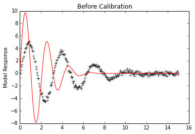
init_vals = p.forward(workdir='initial',reuse_dirs=True)
#f, (ax1,ax2) = plt.subplots(2,sharex=True)
plt.plot(x,data, 'k+')
plt.plot(x,p.simvalues, 'r')
plt.ylabel("Model Response")
plt.title("Before Calibration")
plt.show()

# Calibrate parameters to data, results are printed to screen
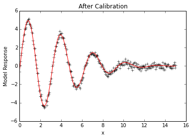
m = p.lmfit(cpus=2,workdir='calib')

[[Variables]]
     amp:       5.011398 +/- 0.040472 (0.81%) initial =  10.000000
     decay:     0.024835 +/- 0.000465 (1.87%) initial =  0.100000
     omega:     1.999116 +/- 0.003345 (0.17%) initial =  3.000000
     shift:    -0.106207 +/- 0.016466 (15.50%) initial =  0.000000
[[Correlations]] (unreported correlations are <  0.100)
    C(omega, shift)              = -0.785
    C(amp, decay)                =  0.584
    C(amp, shift)                = -0.117
None
SSR:  12.8161380426

# Look at calibrated fit
plt.plot(x,data, 'k+')
plt.plot(x,p.simvalues, 'r')
plt.ylabel("Model Response")
plt.xlabel("x")
plt.title("After Calibration")
plt.show()

Template file (sine.tpl) used by pest_io.tpl_write (refer to run_extern function above). Note the header ptf % and parameter locations indicated by % in the file.

DOWNLOAD MODEL TEMPLATE FILE

ptf %
import numpy as np
import cPickle as pickle

# define objective function: returns the array to be minimized
def sine_decay():
    """ model decaying sine wave, subtract data"""
    amp = %amp%
    shift = %shift%
    omega = %omega%
    decay = %decay%

    x = np.linspace(0, 15, 301)
    model = amp * np.sin(x * omega + shift) * np.exp(-x*x*decay)

    obsnames = ['obs'+str(i) for i in range(1,model.shape[0]+1)]
    return dict(zip(obsnames,model))


if __name__== "__main__":
    out = sine_decay()
    pickle.dump(out,open('sine.pkl', 'wb'))