Sampling

This example demonstrates a Latin Hypercube Sampling of a 4 parameter 5 response model using the lhs function. The models of the parameter study are run using the run function. The generation of diagnostic plots is demonstrated using hist, panels, and corr.

%matplotlib inline
import sys,os
try:
    import matk
except:
    try:
        sys.path.append(os.path.join('..','src'))
        import matk
    except ImportError as err:
        print 'Unable to load MATK module: '+str(err)
import numpy
from scipy import arange, randn, exp
from multiprocessing import freeze_support

# Model function
def dbexpl(p):
    t=arange(0,100,20.)
    y =  (p['par1']*exp(-p['par2']*t) + p['par3']*exp(-p['par4']*t))
    #nm =  ['o1','o2','o3','o4','o5']
    #return dict(zip(nm,y))
    return y

# Setup MATK model with parameters
p = matk.matk(model=dbexpl)
p.add_par('par1',min=0,max=1)
p.add_par('par2',min=0,max=0.2)
p.add_par('par3',min=0,max=1)
p.add_par('par4',min=0,max=0.2)

# Create LHS sample
s = p.lhs(siz=500, seed=1000)

# Look at sample parameter histograms, correlations, and panels
out = s.samples.hist(ncols=2,title='Parameter Histograms by Counts')

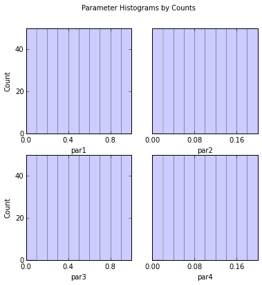
par1:
Count:           50       50       50       50       50       50       50       50       50       50
 Bins:        0      0.1      0.2      0.3      0.4      0.5      0.6      0.7      0.8      0.9        1

par2:
Count:           50       50       50       50       50       50       50       50       50       50
 Bins:        0     0.02     0.04     0.06     0.08      0.1     0.12     0.14     0.16     0.18      0.2

par3:
Count:           50       50       50       50       50       50       50       50       50       50
 Bins:        0      0.1      0.2      0.3      0.4      0.5      0.6      0.7      0.8      0.9        1

par4:
Count:           50       50       50       50       50       50       50       50       50       50
 Bins:        0     0.02     0.04     0.06     0.08      0.1     0.12     0.14     0.16     0.18      0.2

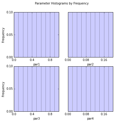
out = s.samples.hist(ncols=2,title='Parameter Histograms by Frequency',frequency=True,printout=False)

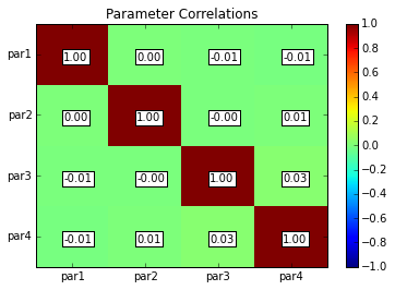
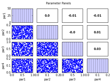
parcor = s.samples.corr(plot=True, title='Parameter Correlations')

             par1     par2     par3     par4
par1         1.00     0.00    -0.01    -0.01
par2         0.00     1.00    -0.00     0.01
par3        -0.01    -0.00     1.00     0.03
par4        -0.01     0.01     0.03     1.00

out = s.samples.panels(title='Parameter Panels')

# Run model with parameter samples
s.run( cpus=2, outfile='results.dat', logfile='log.dat',verbose=False)

# Look at response histograms, correlations, and panels
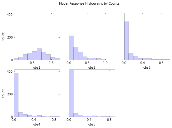
out = s.responses.hist(ncols=3,title='Model Response Histograms by Counts', printout=False)

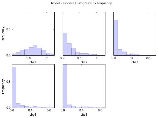
out = s.responses.hist(ncols=3,title='Model Response Histograms by Frequency',frequency=True,printout=False)

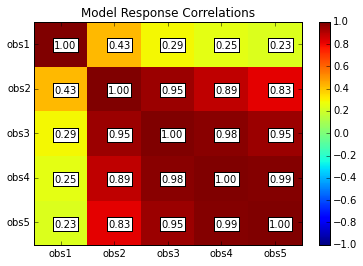
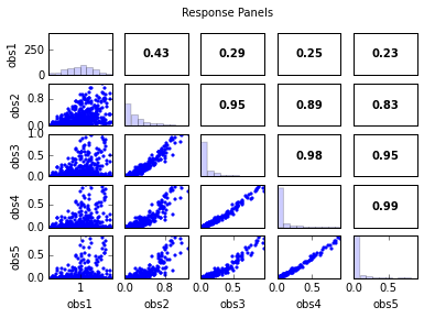
rescor = s.responses.corr(plot=True, title='Model Response Correlations')

             obs1     obs2     obs3     obs4     obs5
obs1         1.00     0.43     0.29     0.25     0.23
obs2         0.43     1.00     0.95     0.89     0.83
obs3         0.29     0.95     1.00     0.98     0.95
obs4         0.25     0.89     0.98     1.00     0.99
obs5         0.23     0.83     0.95     0.99     1.00

out = s.responses.panels(title='Response Panels')

# Print and plot parameter/response correlations
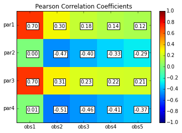
print "\nPearson Correlation Coefficients:"
pcorr = s.corr(plot=True,title='Pearson Correlation Coefficients')

Pearson Correlation Coefficients:
             obs1     obs2     obs3     obs4     obs5
par1         0.70     0.30     0.18     0.14     0.12
par2         0.00    -0.47    -0.40    -0.33    -0.29
par3         0.70     0.31     0.23     0.22     0.21
par4         0.01    -0.51    -0.46    -0.41    -0.37

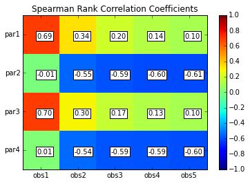
scorr = s.corr(plot=True,type='spearman',title='Spearman Rank Correlation Coefficients',printout=False)

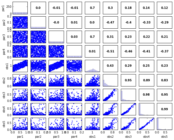
out = s.panels(figsize=(10,8))